Butterfly valve control with an S7 1200 Controller
This blog covers how to control a valve with the Siemens S7-1200 controller. I have tried to keep it simple yet cover everything from the wiring through to the PLC program and HMI Design. This blog is divided into 3 parts, the first will be the physical connection, the second the ladder program and finally in the third part, a HMI that allows user manipulation of the valve. I thoroughly enjoyed getting the time to do this and thank you to Alan Phillips for providing the 2 days requested to complete it.
Part 1 - Physical connections
First of all, we need to identify the valve we want to operate. In this case the valve belongs to the company Promation. I chose the valve “P2/3 HV AC Series”, because it meets torque needs for a project I am currently working on.
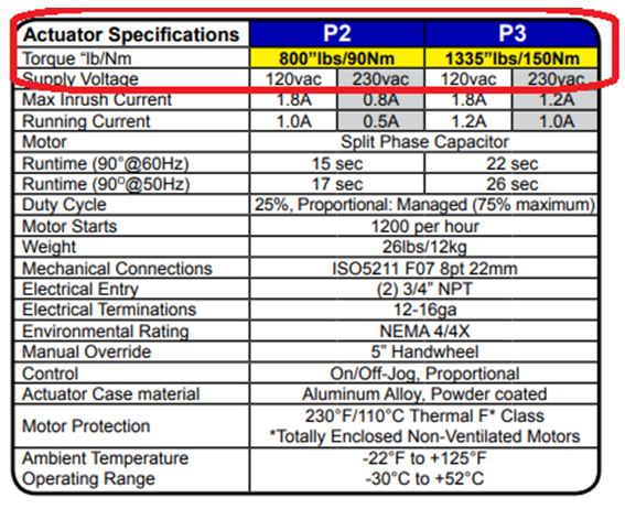
Figure 1. Actuator Specifications.
In order to carry out an automation project, we must first identify the voltages with which our actuators and sensors work. All this information is located on Datasheets are normally supplied by the manufacturer. In this case it was (https://www.promationei.com/technical.cfm)
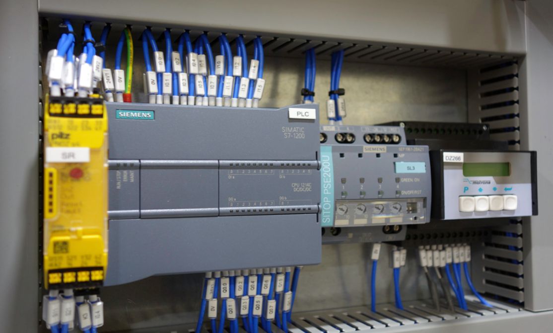
Once the actuator has been identified, we proceed to identify the controller. In this case I used the SIEMENS S7 1200 controller. Because it is simply the one we have available, and since it is only a valve that will be controlled, it is only necessary to have 1 digital output card, but for larger projects it is necessary to check the amount of digital inputs and outputs as well as the analog ones. The model of the controller was “6ES7215-1BG40-0XB0”. If we look for information about this equipment on the website of its manufacturer (https://mall.industry.siemens.com/) we will find the following.
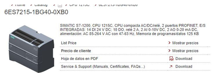
Figure 2. Controller Description.
As you can see, in Figure 2, This controller has 14 Digital Inputs that works with 24VDC. It has 10 Digital Outputs, that work with 24 VDC like the Digital Inputs, and the controller has 2 Analog Inputs too. The controller commands Outputs with 24VDC and our actuator works with 230 VAC. To solve this, we will use a relay as an intermediate between the controller and the valve.
We can use any brand that we want, but in this occasion, we choose the model “PLC-RSC- 24DC/21 – 2966171” from the Phoenix Contact company
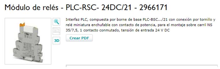
Figure 3. Relay.
This relay works with 24VDC as an input.
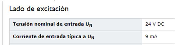
Figure 4. Relay Nominal Voltage Input.
This can support 250VAC as an Output.
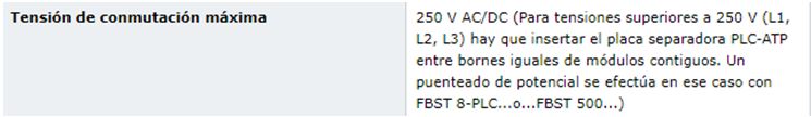
Figure 5. Relay Maximum Switching Voltage. Now we have identified the three main components. Now we need to know how we are going to connect them to each other. For this we return to the Valve’s datasheet.
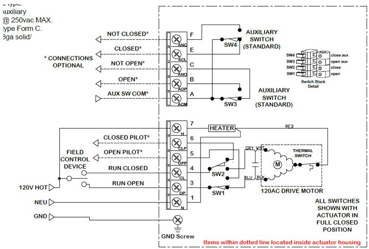
Figure 6. Valve Wiring Indications.
Figure 7. Valve Terminal Blocks.
As you can see on Figure 7. There are 12 Terminal Blocks. Terminal Blocks from 1 to 7 are to the valve control, and Terminal Blocks from A to F are to the valve supervision. Terminal Block 1 and 7 are to feed the Heater. We usually use Heaters when the valve works in humid or very cold environments. Terminal Blocks 5 and 6 are normally connected to Pilot LEDs to indicate the order that is being received from the controller. And finally, Terminal Blocks 3 and 4, they are used to receive the command signal from the controller, having terminal block 1 as common as well as the heater. This means that when we feed Terminal Block 4, the valve will close and when we feed Terminal Block 3 the valve will open. For this project we will only use terminal blocks 1, 3 and 4.Now let’s analyze the relay.
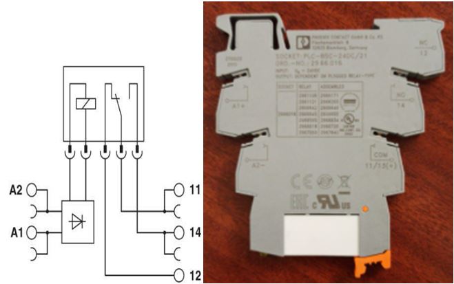
Figure 8. Relay Electrical Diagram.
We can see, how the relay works, output 14 and 12 are normally connected and when we feed the input, output 14 and 11 will be connected. It means we can use the normal position (14 and 12 connected) to keep the valve in a resting state (open) and when we power the relay, the valve will change position (closed).Now let’s analyze the controller.
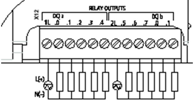
Figure 9. Digital Output Wiring.
As we can see in Figure 10, we have 10 outputs, 1L is the Voltage supply, who receives 24VDC and when we command from the program to the controller to activate an output the internal relay of the controller will close sending 24VDC. So, it means, we need two connections, 1L and any Output in this case A.0.
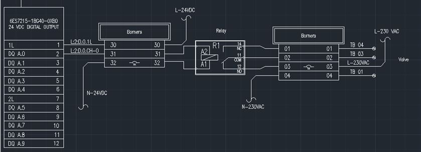
Figure 10. Electrical Wiring.
We can see the Electrical Wiring from the controller going to through the relay to finally end on the valve. As we can see, in Figure 11 there are items called Borners. They are used to order the wiring on the control cabinets and they are Terminal Blocks. We are using two terminal blocks in this example. The first one is: NSYTRV62 from the brand SCHNEIDER.
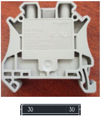
Figure 11. Terminal Block
This Terminal Block is used to connect two points in a system. The second one is: NSYTRV42SF5 from SCHNEIDER too.
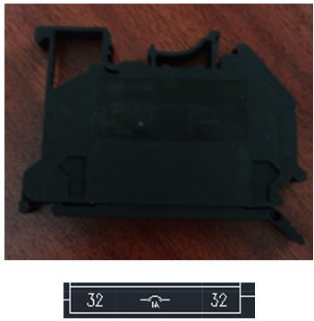
Figure 12. Fuse Holder.
This Terminal Block is used to connect two points and when an overcharge can represent a risk for the circuit.
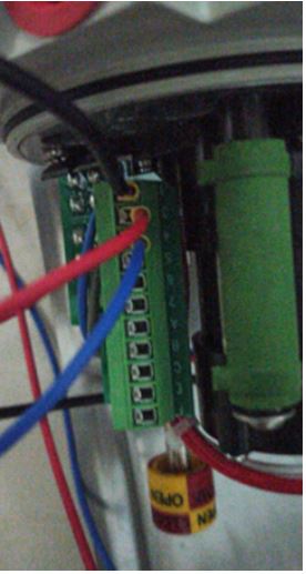
Figure 13. Valve Wired.
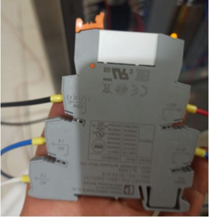
Figure 14. Relay Wired.
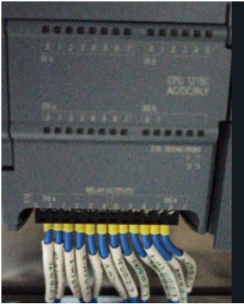
Figure 15. Controller Wired.
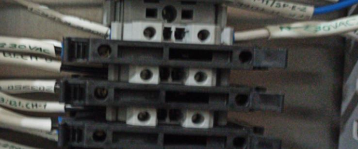
Figure 16. Terminal Blocks Wired.
When everything has been correctly connected, we can proceed to the next part, which is the program design.
Part 2 - S7 TIA PLC Program Design
To get started we must make sure we have the correct program. So we check the equipment data sheet “6ES7215-1BG40-0XB0” , on the manufacturer’s page (https://mall.industry.siemens.com/mall/es/WW/Catalog/Product/6ES7215-1BG40-0XB0) we can download the data sheet.
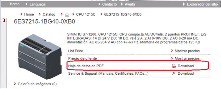
Figure 17. Manufacturer’s page.
Once downloaded we proceed to review it.
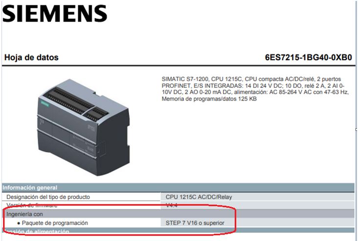
Figure 18. Programming package.
The software and the version with which this equipment can be programmed are highlighted. It is STEP 7 V16 or higher. So, we must make sure we have this software installed. Once installed we proceed to open it.

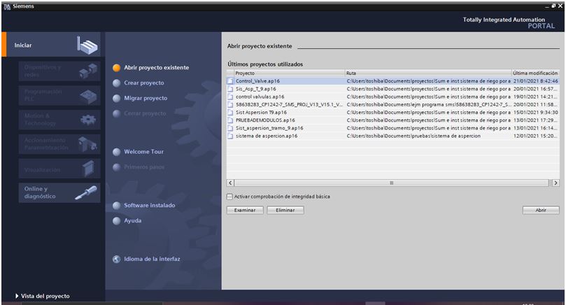
Figure 19. TIA Portal V16.
In this window we can see some projects already created, but we will create one. So, click on “Create project”.
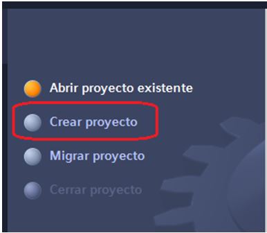
Figure 20. Create a new project.
The following box will appear.

Figure 21. Project creation Settings.
We must complete this box with the project name, the path where the project will be saved and the Author. Then click on “Create”.
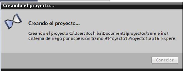
Figure 22. Project being created.
After waiting some seconds, the following box will appear.
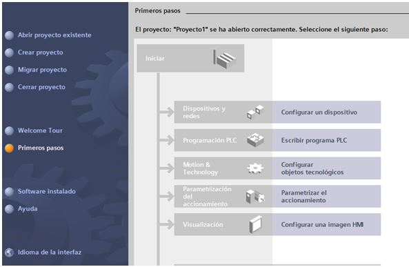
Figure 23. First steps.
On figure 23, we can see different options. The first one, is about to configuration of devices. We will choose this option because it is the first thing we must do. So, click on Configure Devices.
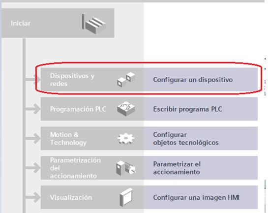
Figure 24. Configure device.
The following box will appear.
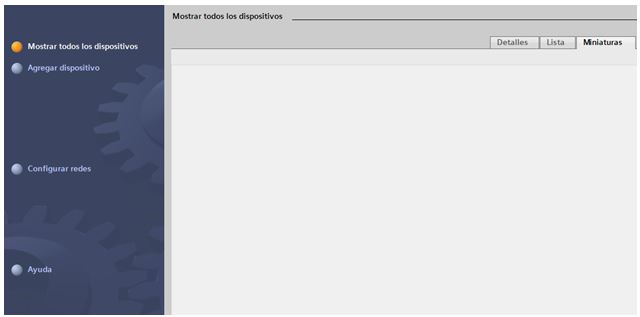
Figure 25. Available Devices.
Click on Add Devices.
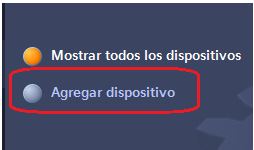
Figure 26. Adding devices.
Now, on the right side, we can see the available Devices.
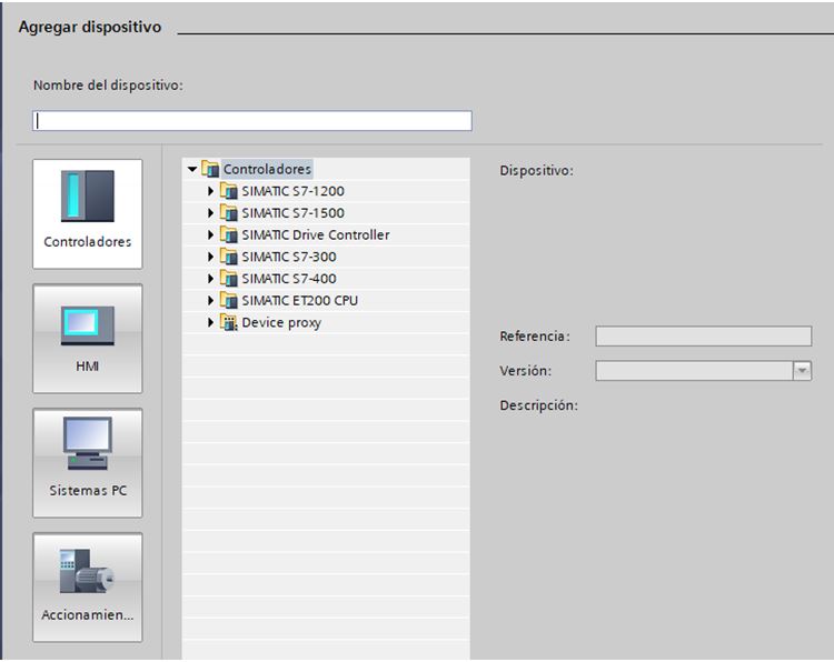
Figure 27. Available Devices.
In this part, we have two options, the first one is, look at the device on the List.
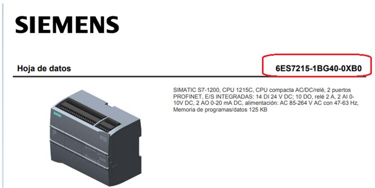
Figure 28. Device Code.
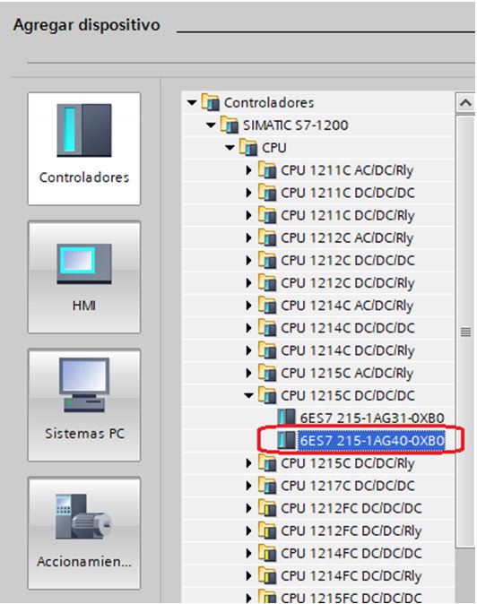
Figure 29. Device located on the controllers List.
Once located and selected we must choose the Version.
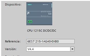
Figure 30. Controller Version.
In this case V4.4, sometimes the controller will have another version, so we will have to update it. Once created click on add.
Figure 31. Add controller to the project. Then, we will be ready to develop the program.
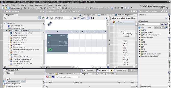
Figure 32. Project ready to be programed.
The second option is to add a generic controller. For this we return to the window where we add devices (Figure 29). We choose an unspecified controller. We choose this option when we do not know the exact model of the controller as well as the current firmware. We need to be physically connected to the controller. In this case my controller has as IP address 192.168.0.1 and my PC has 192.168.0.67.
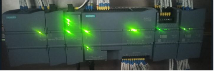
Figure 33. Controller S7 1200.
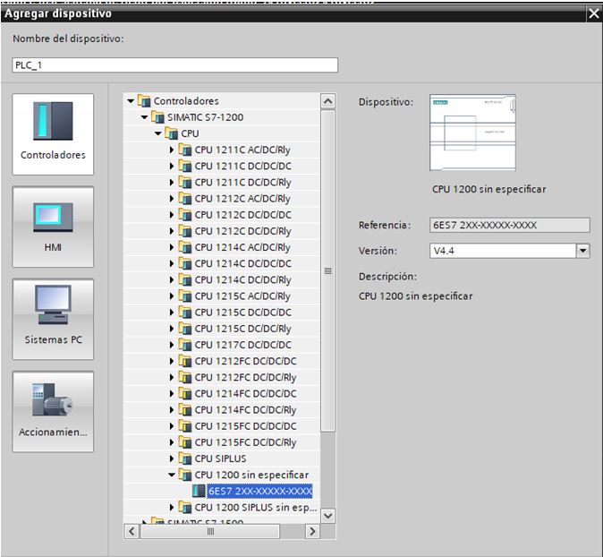
Figure 34. Adding an unspecified controller.
Once selected, click on add.

Figure 35. Add unspecified controller to the project.
Once added, the following window will appear.
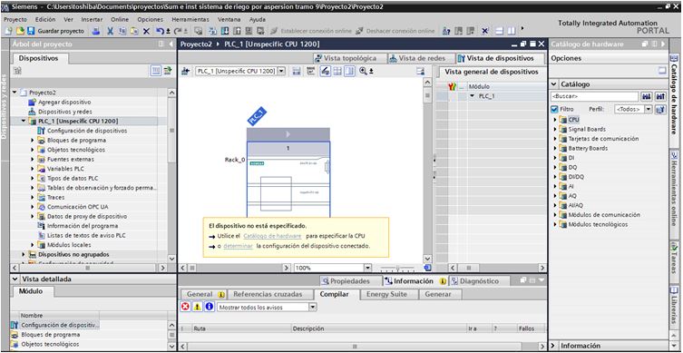
Figure 36. Unspecified controller added to the project.
Notice the dialog box down the unspecified controller.
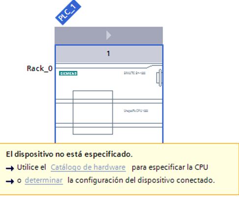
Figure 37. Unspecified controller’s dialog box.
TIA Portal is asking us to define the controller, and gives us two options to do it. The first one is to use Hardware Catalogue; we already developed this method previously. The second option is to determine the configuration based on the one we have connected. Lets click on this option “decide”. The following window will appear.
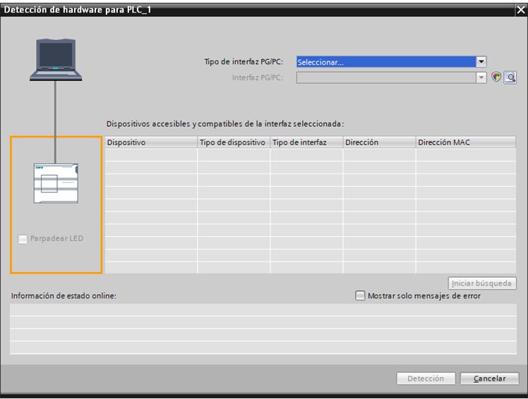
Figure 38. Hardware Detection.
On interface type select PN/IE
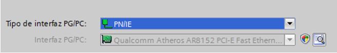
Figure 39. Interface PG/PC. Now, click on “star search”.
Figure 40. Star search.
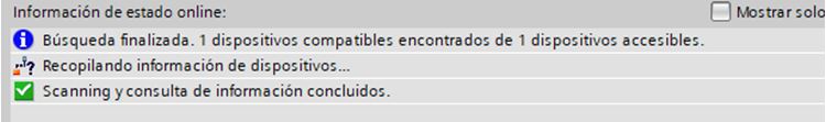
Figure 41. Device Identified.
As we can see , there is one device found. Once the device is found we click on detect.
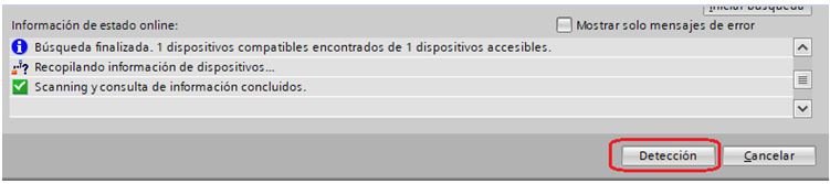
Figure 42. Detect Device.
This action will return us to the window . The device configuration will be loaded based on the one detected.
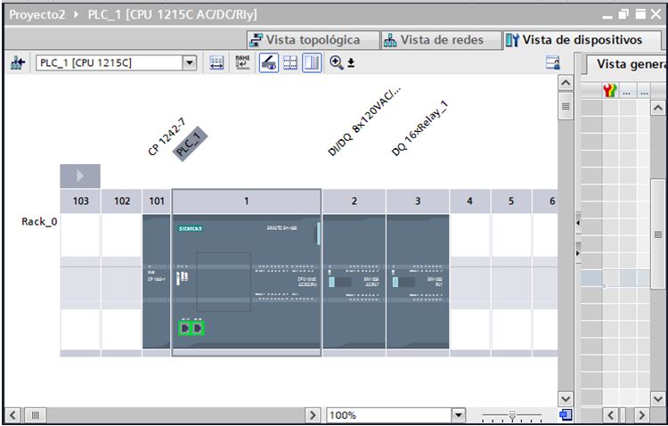
Figure 43. Device configuration loaded.
We can see more devices apart from the controller. This is because these devices physically exist as seen in figure 33. So, this is a good method to detect what you have online. Now select the controller clicking on it.
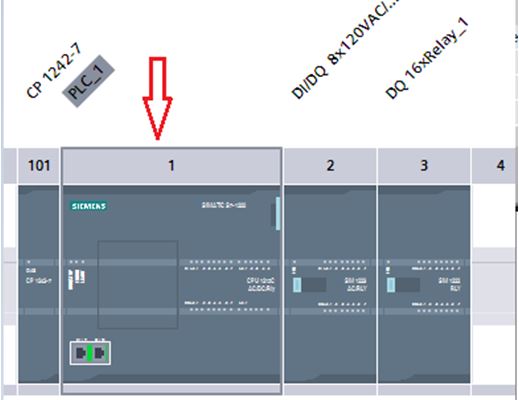
Figure 44. Selecting controller. At the bottom we find the properties of it.
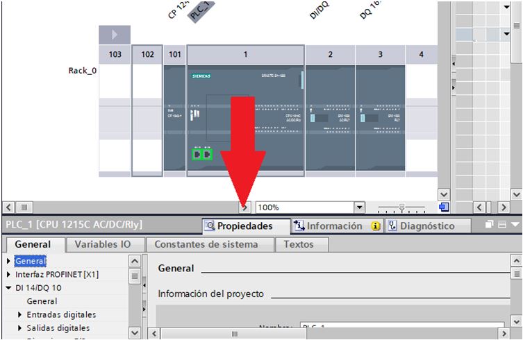
Figure 45. Controller properties.
Let’s expand this box so we can review it more easily.
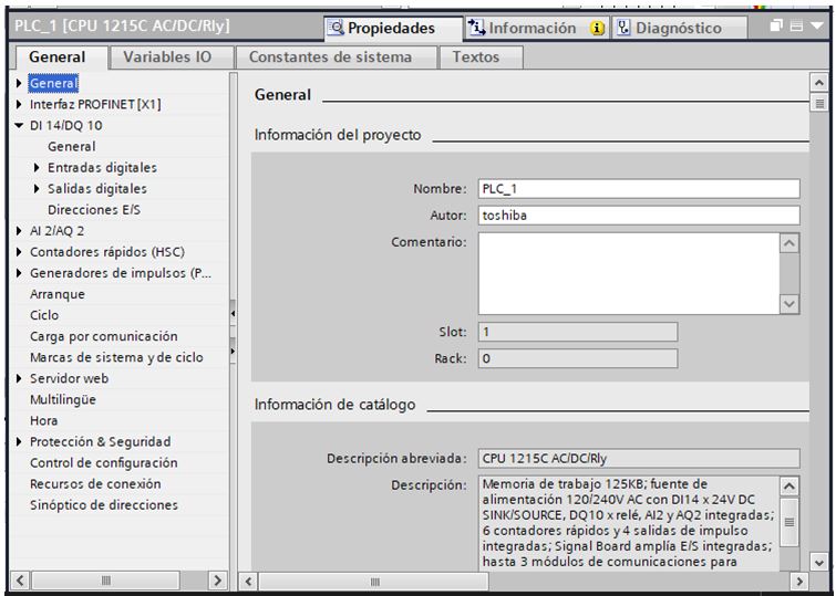
Figure 46. Controller properties box expanded. Now let’s explore the principal properties of this controller, first, the firmware version.
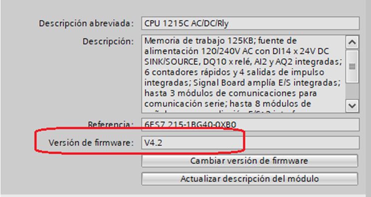
Figure 47. Firmware Version. But more importantly, check the addresses of our digital outputs, which we will use to control the valve.
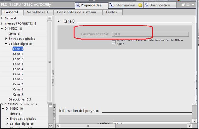
Figure 48. Digital Output Address.
We can see that the first digital output has the address Q0.0. We will use this address to control the valve. Once identified we return to the project tree. Then we select “Program Blocks”.
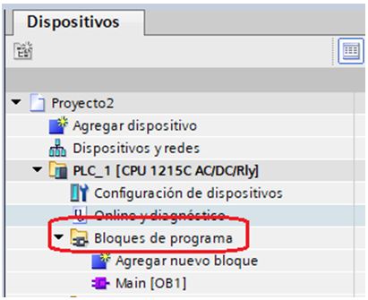
Figure 49. Program Blocks.
Then click on “Main OB1”, this is the principal subroutine. The following window will appear.
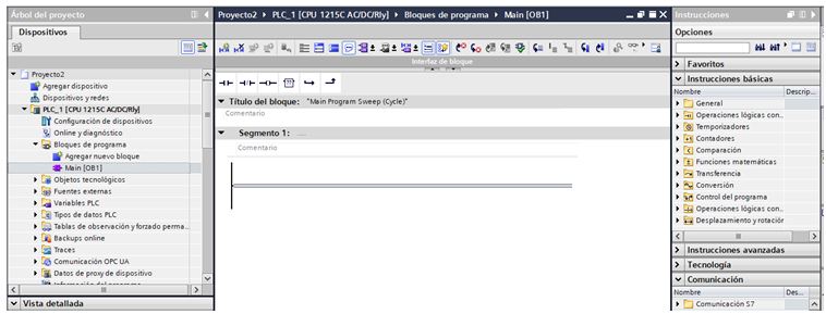
Figure 50.Main OB1.We will develop the program here. This is a ladder environment. We will create a simple Program. We need a normally opened contact controlled by a memory bit, because we don’t have any physically button. For this we drag this contact from the block menu to the ladder line.
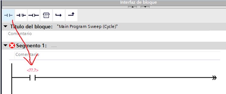
Figure 51. Normally Opened contact inserted on the ladder program.
Now, we must assign this contact to a bit memory. So, lets create some variables first. On the Tree project select and click “variable table”, that is located under “PLC variables”.
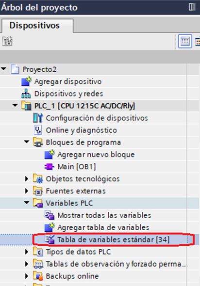
Figure 52. Opening Variable Table.
The following window will appear.
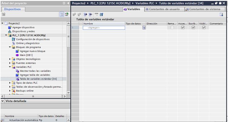
Figure 53. Variable Table.
In this window, we can create variables that will be used on the program. First, we create two variables, assigned to memory bits as we will use them to make the control.
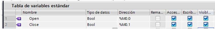
Figure 54. Control Variables.
Now we will create an Output Tag, assigned to the output direction that we identified.
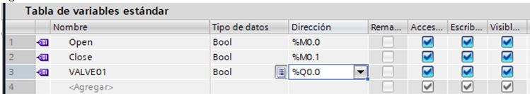
Figure 55. Output variable created.
Now return to the MAIN OB1 and assign to the normally opened contact the “open variable”.
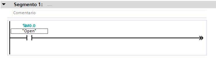
Figure 56. Open variable assigned to the contact.
Now drag an output to the ladder.
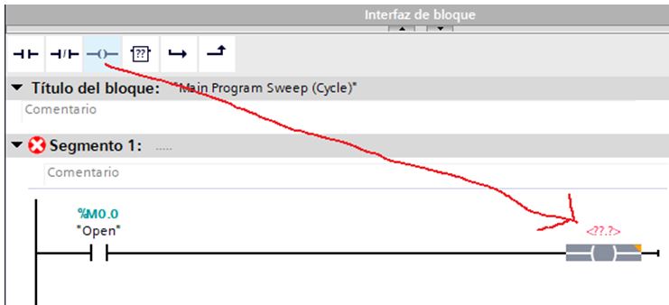
Figure 57. Output dragged to ladder program.
Assign to the output to the “valveo1” TAG.
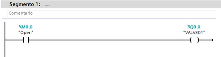
Figure 58. Ladder program with variables assigned.
Now there is a problem, the VALVE01 will be activated meanwhile the normally open contact is closed, but we need to lock this, so let’s configure the program as follows.
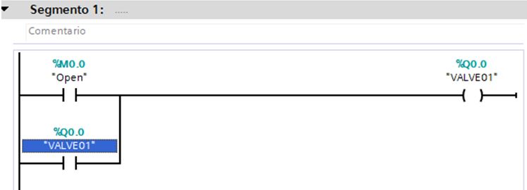
Figure 59. VALVE01 locked.
Now the VALVE01 output will remain activated. But there is a problem again, what about if we want to deactivate it? We need to add a new contact but now It will be normally close.
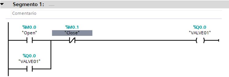
Figure 60. Normally Closed Contact inserted an assigned.
Now our program is ready to work, we can open the valve with the “open” contact, and close it with “close” contact. So, let’s try it. For that we need to compile it. Click on compile icon.
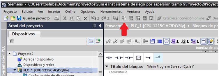
Figure 61. Compile icon.
We will see a report of the compilation at the bottom.
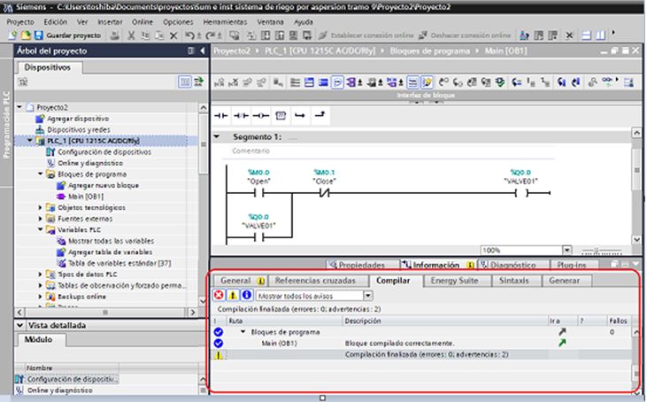
Figure 62. Compilation report.
As we can see , there is no errors on the compilation. We can download the program to the controller. For that click on download icon.
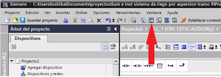
Figure 63. Download Icon.
The following window will appear.
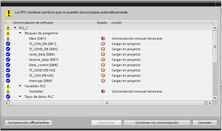
Figure 64. Download Window.
Click on continuing without synchronization.
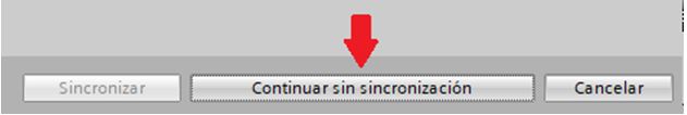
Figure 65. Continuing without synchronization.
The following window will appear
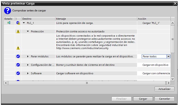
Figure 66. Preliminary view to the download.
Click on “load”.
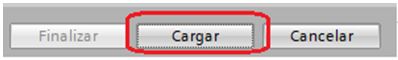
Figure 67. Download.
The following window will appear.
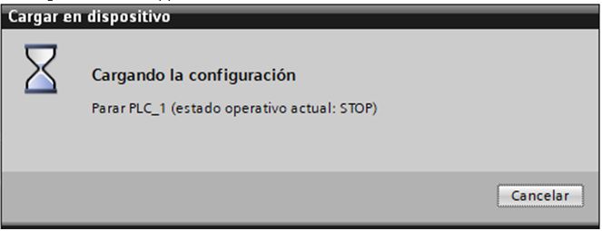
Figure 68. Loading configuration. The following window will appear.
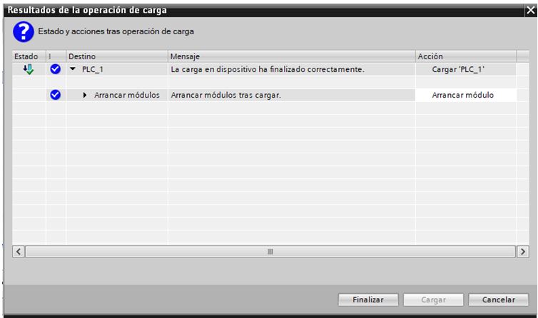
Figure 69. Loading Results.
Click on Finalize.
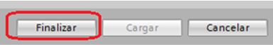
Figure 70. Finish Load.
Now the program is loaded, let’s stablish connection with the controller to monitor the program online. For that click on “Establish online connection”.
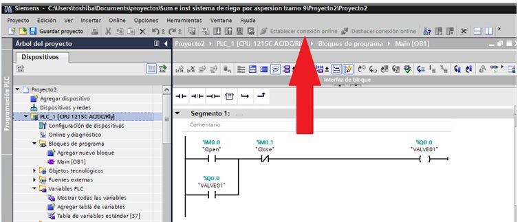
Figure 71. Online connection option.
We will notice that it is online by the green Icons and the orange line.
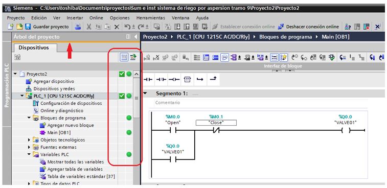
Figure 72. Online connection whit the controller.
Now click on observation icon to see how is the program running.
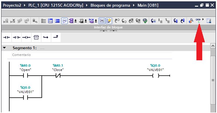
Figure 73. Observed Ladder Program.
Now let’s control the valve, for that we need to toggle the contacts. So right click on open contact and choose force.
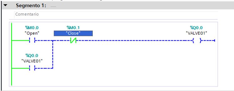
Figure 74. Forcing “OPEN” contact.
Now force it to 1.
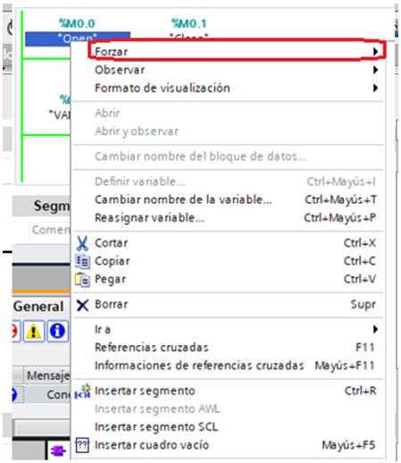
Figure 75. Forcing “OPEN” contact to 1. Once Forced, the output will be activated.
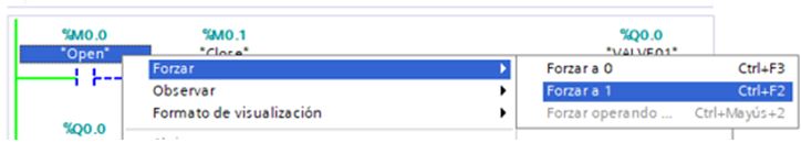
Figure 76. Output activated.
A LED will light on the controller indicating the active output.
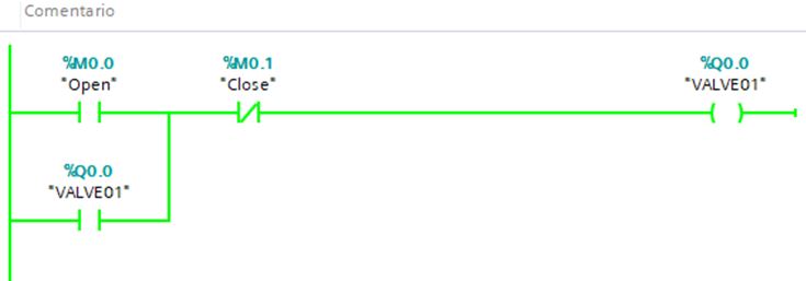
Figure 77. Indicative LED on.
And the actuator will be activated.
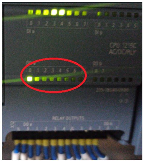
Figure 78. Open valve.
Now let’s close the valve. Force Normally Close Contact for that.
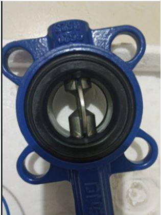
Figure 79. Forcing Normally Close Contact to 1. Now the output is disactivated.
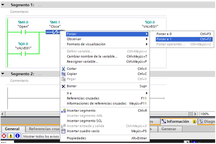
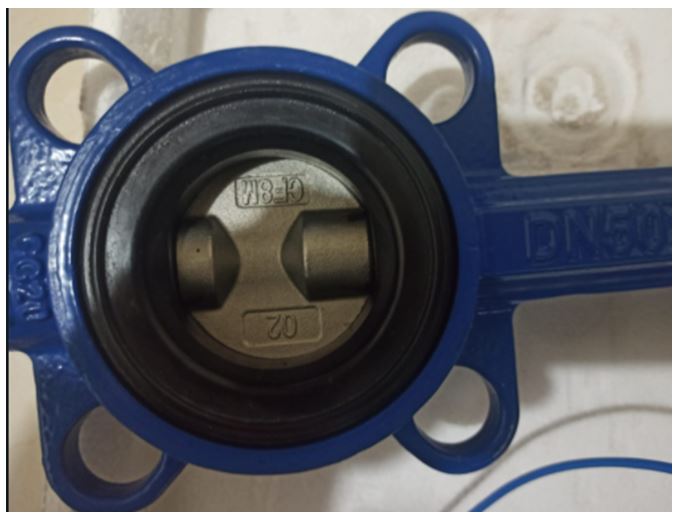
Figure 80. Output Disactivated. Now the valve is closed.
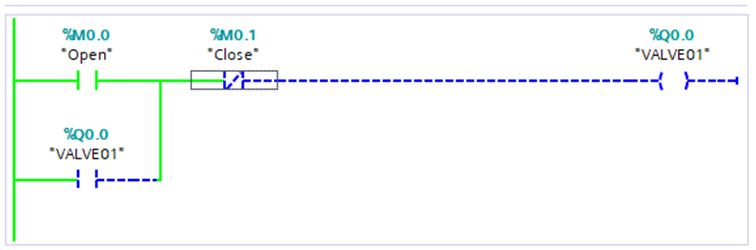
Figure 81. Closed Valve.
Now we know how to control a valve with a ladder program. Next to the HMI.
Part 3 - WinCC HMI Design
To add the HMI to our project, we return to the tree project, and click on Add Device.
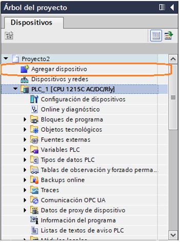
Figure 82. Adding a device into the project.
Now, we are adding and HMI, so we select that option.
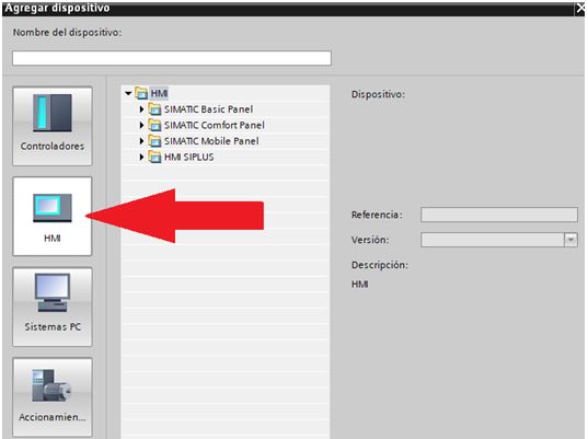
Figure 83. Selecting the HMI’s List.
In our case we have, an KTP400 BASIC PANEL, and his product code is “6AV2123-2DB03-0AX0”, So we look it up on the HMI’s list.
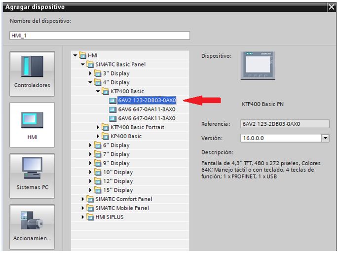
Figure 84. Selecting 6AV2123-2DB03-0AX0. Now click on Accept.
The following assistant will appear.
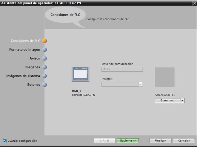
Figure 85. HMI’s assistant.
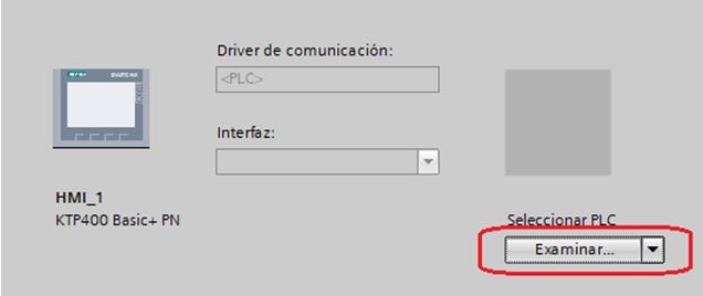
Figure 86. Selecting an PLC.
This Option will allow us to decide with which PLC to connect with.
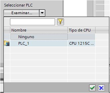
Figure 87. Available PLC’s list.
We can see 1 PLC available, but in larger projects we could have more PLCs. Now, let’s select the one we have and click on check.
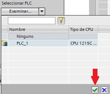
Figure 88. Selecting an PLC.
Now the PLC has been identified and the Profinet connection too.
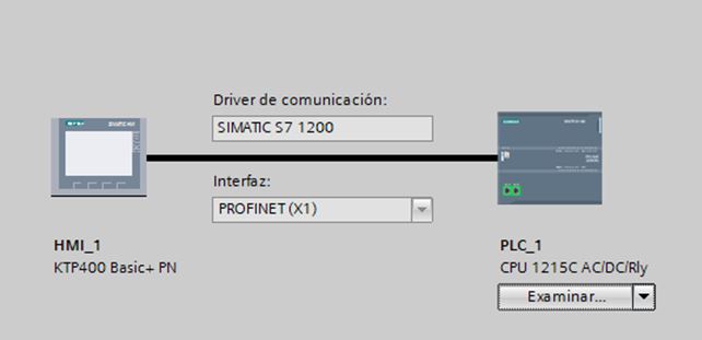
Figure 89. HMI and Profinet connection identified.
Click on next.
Figure 90. Next.
The following window will appear.
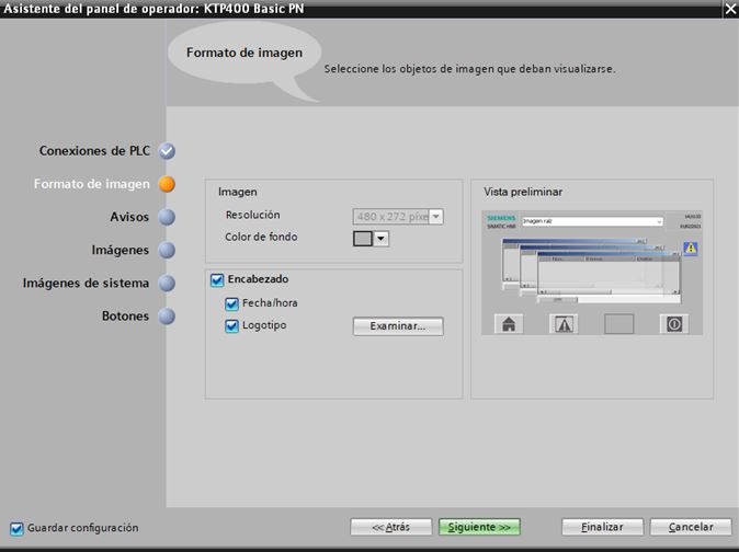
Figure 91. Image Format.
We can configure the background color and the header. Let’s change the background from gray to white, and remove type from the header.
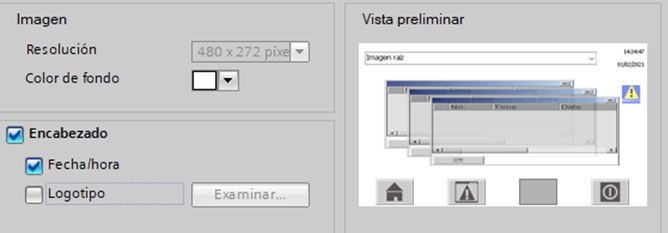
Figure 92. Background and Header configured.
Now click on next.
Figure 93. Next to advices.
The following window will appear.
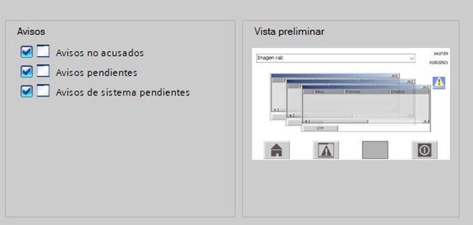
Figure 94. Advices.
On figure 87 we can configure the advices for when we have alarms. That isn’t our case, so click on Next.

Figure 95. Images.
In this part you can define how many screens there will be and their hierarchy. In our case we will have only one, the main. So click on next.
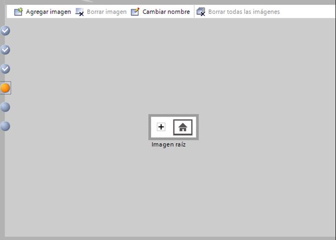
Figure 96. Next to System images.
The following window will appear.

Figure 97. System images. On this part, we can configure some tools to the HMI. For example the diagnostic viewer, project information, etc. Click on Next.
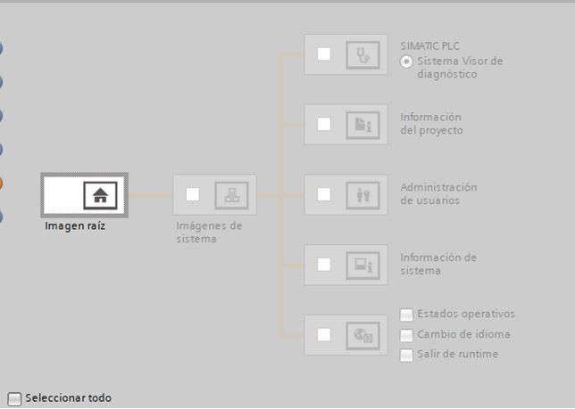
Figure 100. Next to Buttons.

Figure 101. Buttons.
On this part, we can configure the function of the physical buttons of the HMI. For example, there are three buttons assigned with defined functions.
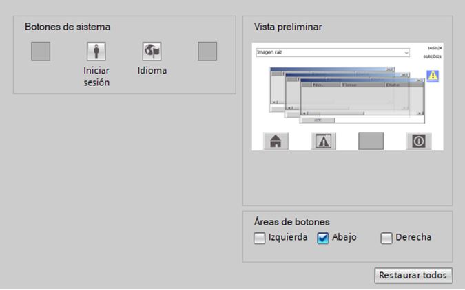
Figure 102. Buttons Assigned.
And two defined functions ready to be assigned.
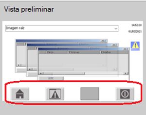
Figure 103. Buttons Unassigned.
In our case, we will use the already defined ones. Click on finalize. The next window will appear.
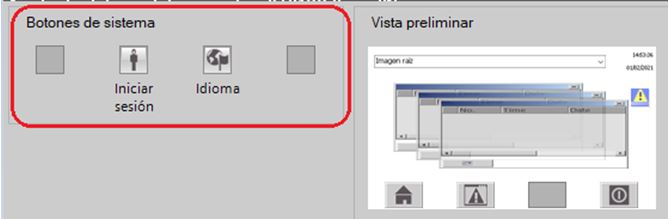
Figure 104. HMI drawing area.
On this area, we can draw our HMI. To do this we will have some tools.
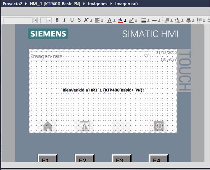
Figure 105. TOOLS to draw an HMI.
As we can see, we have limited tools to draw because the HMI to use is a basic one, but they are enough for our application. So, let’s Draw a symbol that represents the valve.
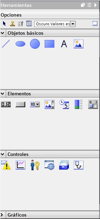
Figure 106. Classic Valve Symbol.
Now let’s add some indicators that show us if the valve is ON or OFF. For example Text and one led that changes color.
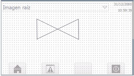
Figure 107.Valve status indicators.
Now let’s add animations to this indicator. For that, double click on them, lets start for text indicators.
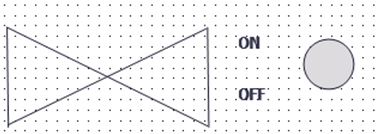
Figure 108. ON Text configuration.
As you can see on figure 100, we are exploring ON text properties, select “animations”.
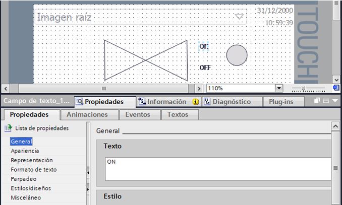
Figure 109. ON Text animations.
Let’s make the ON text display when the valve has been commanded to open. So, click on add animation.
Figure 110. Adding animation to ON text.
The following window will appear. Select visibility and click on Accept.
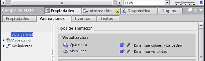
Figure 111. Adding visibility animation to ON text.
The following window will appear.
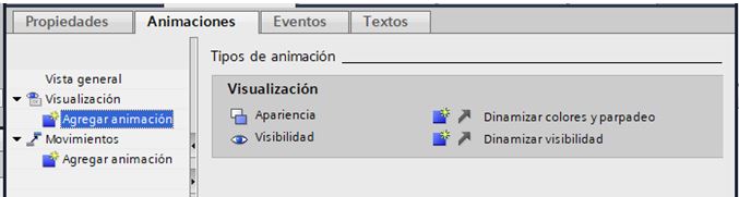
Figure 112. Adding visibility animation to ON text.
We can assign which variable will control the animation. So click on variable search menu.
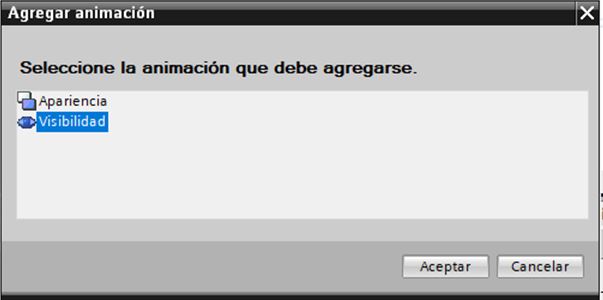
Figure 113.Selecting variable.
Look the variable on the explorer.
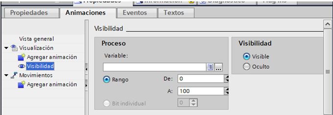
Figure 114. Select VALVE01 variable.
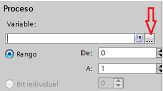
Figure 115. VALVE01 variable selected.
Do the same for OFF text, but, instead visible select hide.
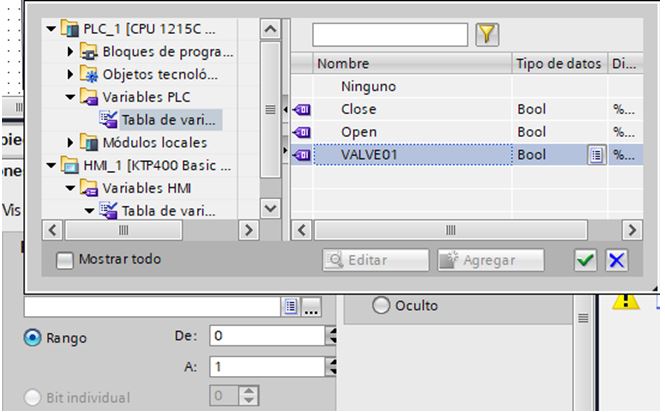
Figure 116. OFF text Hide.
Do the same with the circle.
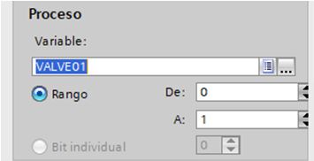
Figure 117. Circle visibility configured.
Now, lets configure the commands to operate the valve. For that we need to insert two buttons, one to open it and one to close it.
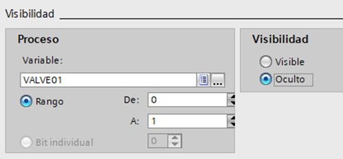
Figure 118.Button tool.
Drag the button tool from the tool’s menu to the HMI. Do this two times because we need two buttons.
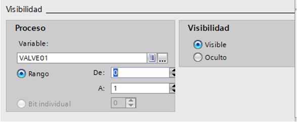
Figure 119. HMI with two buttons.
Configure text double clicking on buttons.
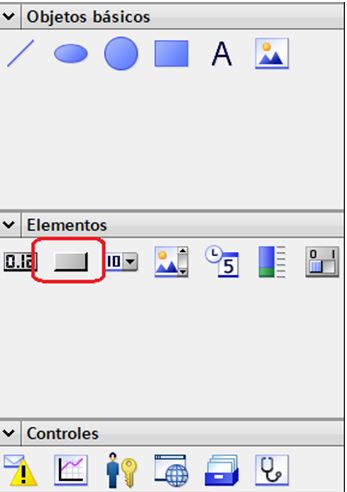
Figure 120. HMI with two buttons.
Now let’s configure the first button, on button, double click on it. Now on menu events, Select the function and assign the variable.
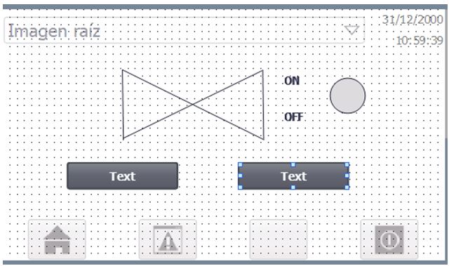
Figure 121.Function assigned to ON button.
Do the same with off button, but assigning close variable.
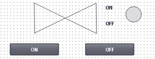
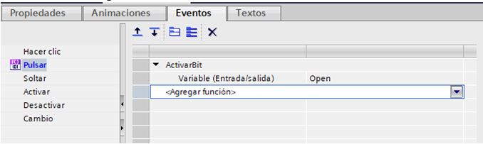
Figure 122. Function assigned to OFF button.
Now our HMI is ready, lets compile it.
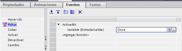
Figure 123.Compile HMI.
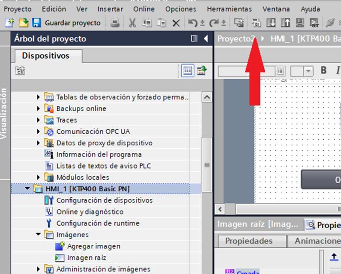
Figure 124. HMI compiling.
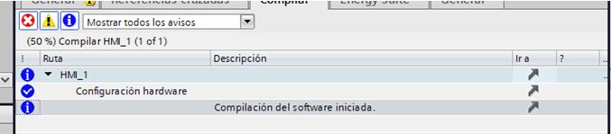
Figure 125. HMI compiled without errors.
Now let’s download the configuration.
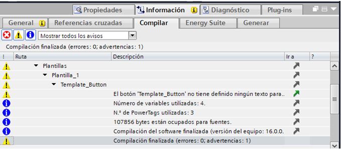
Figure 126.Download HMI configuration.
The following window will appear.
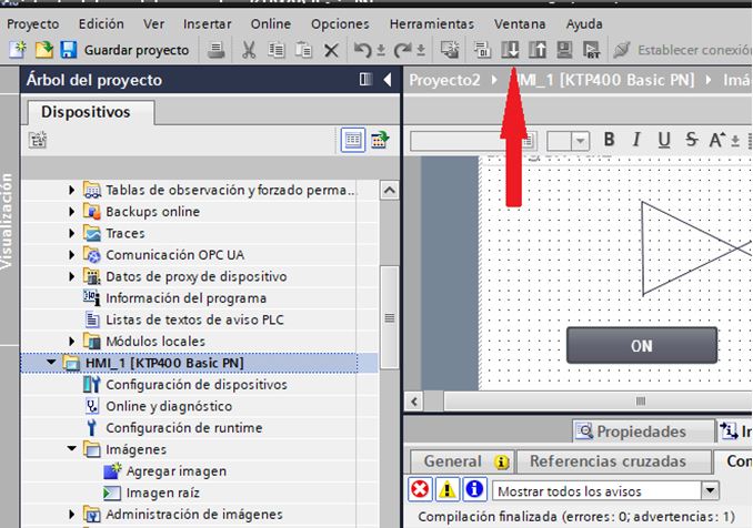
Figure 127. Identifying HMI.
Select, Interface and Ethernet driver.
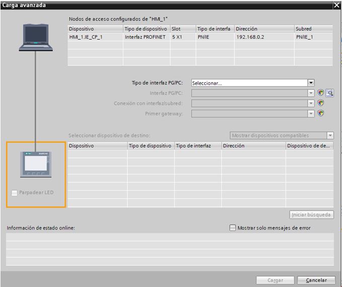
Figure 128.Interface and driver selected.
Now click on “Star Search”.
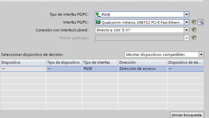
Figure 129.Panel View Detected.
Before we continue, I need to indicate that the panel view is physically connected to the controller. Via Ethernet cable. Ok once the Panel view has been identified click on charge.
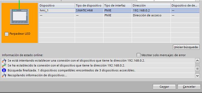
Figure 130.Preparing charge operation.
The following window will appear.
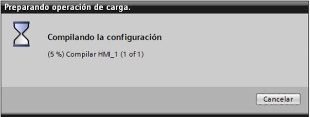
Figure 131.Preliminary charge view. Click on charge.
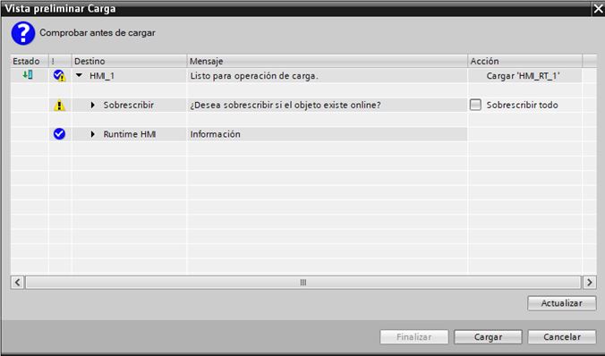
Figure 132.Charging operation completed.
Now the download has been completed.
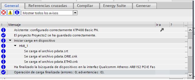
Figure 133. Panel View configured.
Now we can control our valve from the Panel View. This configuration only works once, because if you followed the instructions as is, you will have noticed that when you try to open or close the valve for the second time it does not work. That is because, we are changing the Bit assigned to the buttons but we aren’t returning them to their original position. So, Let’s return to ON button configuration. Select Events menu, Now, on release add a new animation “disactivate bit”.
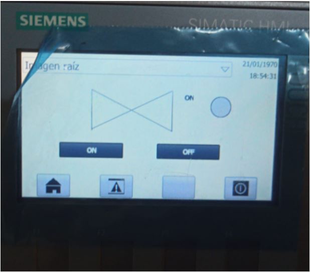
Figure 134. Adding event to ON button.
Now, with this event added, when we release the button, the variable will return to its original position, do the same with the OFF button.
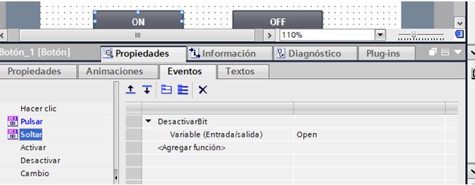
Figure 135. Adding event to OFF button.
Once we do this, repeat the compile and download process, now our HMI will control the valve correctly. Now ON text, OFF text and Circle aren’t working, so let’s try another configuration. First let’s delete the existing animation. For that, select it, right click and delete it.
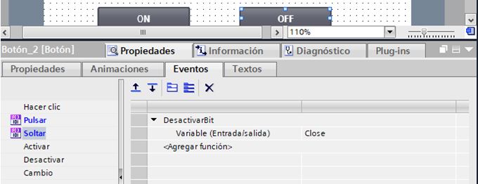
Figure 136. Deleting visibility animation.
Do the same for OFF text and circle. Now let’s add a new animation, but now, appearance animation. Let’s configure it as follows.
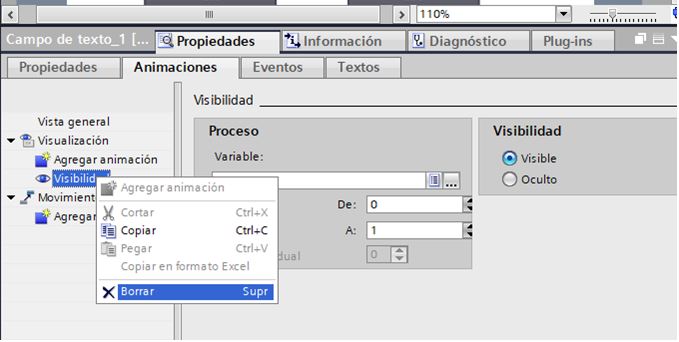
Figure 137. ON appearance configuration.
Do the same for circle and configure OFF text as follows.
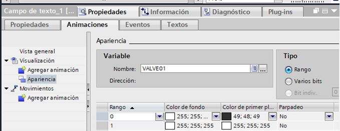
Figure 138. OFF appearance configuration.
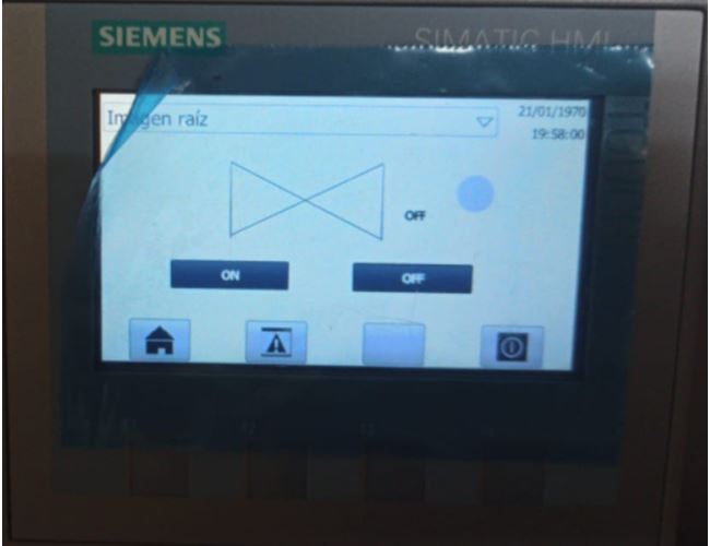
Now, compile and download. Now animations work fine.
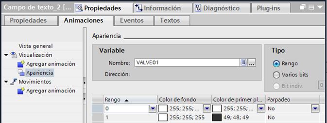
Figure 139. OFF Animation.
Thank you for reading through this blog Article. If you have any questions please reach out to:
contact@appliedprojectsengineering.com
